
Is a compute crunch coming?
We estimated trends in global inference capacity and found that token demand appears to be growing much faster than supply.
Gradient Updates shares more opinionated or informal takes on big questions in AI progress. These posts solely represent the views of the authors, and do not necessarily reflect the views of Epoch AI as a whole.
Much has been made about AI-driven capex in the past year. Hyperscalers have been clamoring to construct massive data centers, spending hundreds of billions in the process. The St. Louis Fed estimates that AI-related investment contributed about 1 percentage point — almost 40% of the total — to US real GDP growth in the first three quarters of 2025, exceeding the IT investment contribution at the height of the dot-com boom. Whether the current AI buildout constitutes a bubble depends largely on whether there will be sufficient demand for the computing infrastructure being built.
It’s tough to estimate future demand for tokens, as it depends heavily on hard-to-forecast trends in capabilities and diffusion. However, we have a much more concrete picture of the supply side. In this article, we do our best to answer how many tokens per second the world could produce with the chips we have today.
To do this, we dig into the technical details of inference. We model prefill and decode runtimes, account for two common efficiency techniques (chunked prefill and speculative decoding), and calibrate against data from SemiAnalysis’s InferenceX, a repository of real-world inference experiments. Our results suggest these chips could serve between 500 million and 20 billion output tokens per second from a Kimi K2.6-like model as of Q4 2025, depending on the context length of requests. We also find that global inference capacity is more than tripling each year, as more computing infrastructure is deployed and chips become more efficient.
We compare these supply estimates to several (imperfect) proxies for token demand and its growth trend, including the growth of tokens served across Google platforms, and the intensity of token usage today at the largest tech companies, extrapolated to all software engineers worldwide. These figures suggest that demand at current prices could be between 200 million and 4 billion tokens per second, growing by roughly 10× per year — plausibly outpacing supply growth in the near future, if not already. However, these estimates are highly uncertain. For one, we don’t know the average size of the models behind current demand. Aggregate token figures also obscure an underlying trend in model efficiency, which both lowers the cost of producing tokens at a given quality, and introduces new demand as additional use cases become cost-effective.
If these trends continue, a compute crunch is likely near — particularly for the long-context workloads that drive agentic AI. This will drive up the price of access to frontier capabilities for those willing to pay, while everyday users shift to cheaper, smaller models. It may also mean that AI companies increase their focus on developing more efficient ways to serve models. Because of efficiency gains, these shifts won’t necessarily mean a regression in the capabilities accessible to everyday users — inference and training efficiency are already improving fast enough that the smaller, cheaper models of tomorrow will quickly match today’s frontier.
Introducing our setting
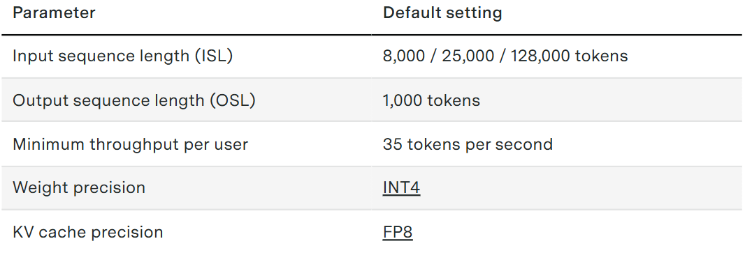
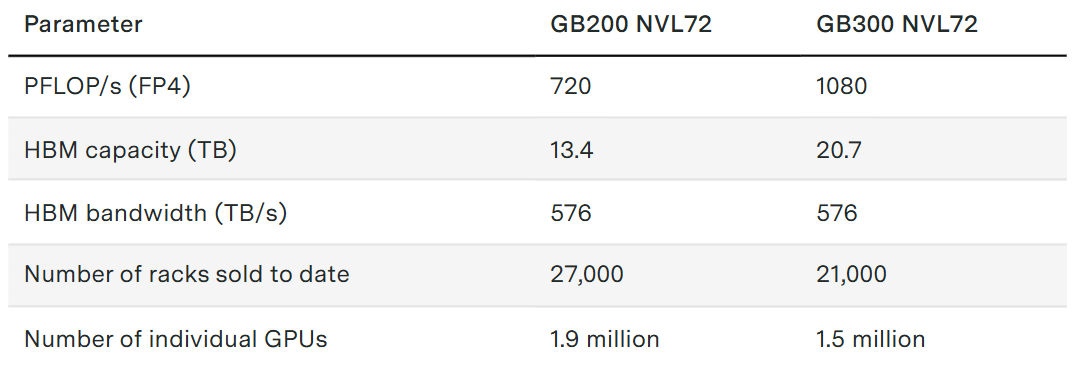
To ground the exercise, we assume we are serving Kimi K2.6 — currently the most capable open model on the Epoch Capabilities Index (ECI)1 — on all of the world’s Nvidia GB200 and GB300 chips (1.9 million and 1.5 million individual GPUs as of Q4 2025, respectively, and representing together roughly 40% of aggregate supply on a FLOP/s basis).
We assume all chips are in NVL72 configurations, where 72 chips are connected per rack. We consider three types of requests: “general” usage (modeled as queries with 8,000 input tokens and 1,000 output tokens), and two longer context settings representing patterns of agentic usage (25,000:1,000 and 128,000:1,000, respectively).2 3 Finally, we assume that users expect at least 35 output tokens per second.4
During our subsequent calculations, we focus on the GB200 systems with 8,000:1,000 query lengths for brevity, applying the same calculations to our GB300s and at each context length to get final figures. It is worth emphasizing that our estimates are contingent on our chosen setting, including the choice of model, numeric format, speculative decoding settings, and many other considerations. We also know little about the architectural details of closed frontier models today, and how they might differ from Kimi K2.6.
Inference settings
Hardware specs
Without further ado, let’s dig into the technical details.
What happens during inference?
AI inference can be broken into two stages: prefill and decoding. During prefill, all input tokens are processed in parallel to populate the “KV cache” — a store of keys and values that allows tokens to attend to previous context without recomputing from scratch each time. Once prefill is complete, the decode stage generates output tokens one at a time, with each new token attending to the cached KVs (and appending its own keys and values to the cache). These two stages have quite different computational properties, so we will look at each in turn.
Our goal in each case is to estimate how long it will take to complete the stage, as a function of important factors like batch size. To do this, we use a simplifying assumption: total time is just whichever is longer — the time it takes to do computations (compute), or the time it takes to move data (bandwidth).
This tends to be a reasonable assumption, for two reasons:
In many cases, one time so dramatically dominates the other that the maximum and the sum are approximately equal.
Even if the two times are similar, they can often happen in parallel. For example, as we process the computations for one layer, the weights for the next layer can already begin to load.
Prefill
Per our assumptions, the prefill stage consists of passing all input tokens through the model to build the KV cache. Language models process many sequences in parallel; we denote the number of concurrent users in each of our NVL72 systems by B, the batch size.
To calculate the prefill compute time ( tcompute ), we count the number of operations that need to be performed per forward pass at each precision and divide by our hardware FLOP/s at the corresponding precision. We need to track precision because weight × activation computations are often done in a lower precision compared to attention calculations.
Each activated weight contributes one multiplication operation and one addition operation per token. Attention adds further operations: for each token of context, in each head and each layer, we perform a multiply and add for every dimension of the query–key dot product and the attention-weighted value sum.
For each of these operations-per-token values, we divide by the corresponding hardware FLOP/s at their respective precisions (4-bit for weights, 8-bit for attention), and sum the result to get the number of seconds per token. Then we multiply by the total number of tokens in the prefill (there are B users, each of which has input_len input tokens).
Plugging in our Kimi K2.6 and GB200 NVL72 numbers, we find that 1B milliseconds are required for computation during 8,000 ISL requests.
Bandwidth is simpler to analyze. In order to actually do the calculations we’ve described above, we must move all 1 trillion of the model weights from high-bandwidth memory (HBM) into tensor cores. Since we’re serving the model in FP4 weights (0.5 bytes per weight), that’s 500 GB of weights.5 After completing the calculations, we also have to write the KV cache for each layer back to HBM — after all, this is the whole point of prefill.
Since we’ve assumed the KV cache is stored in FP8 (1 byte per value), this results in 280B megabytes. Adding this to our 500 GB of weights and dividing by our HBM bandwidth, the final time required for data movement in prefill is on the order of 0.9 + 0.0005B milliseconds.
Decode
Compared to prefill, there are four main differences during decoding. First, because tokens are processed sequentially, we have to do a full weight read for each input. Second, we must also read in the KV cache for each token. Third, our computations are now only for a single token, rather than a whole set of tokens in parallel. Each of these factors shifts decoding towards being bandwidth-bound. The fourth factor (KV projection absorption, see below) pushes in the compute-bound direction, but not enough to outweigh the other factors.
Our calculations here will be familiar from prefill. flops_per_token_weights is nearly unchanged from prefill, except that the average context length is now input_length + output_length/2.
One subtle difference in decoding: FLOP_per_token_attn becomes somewhat more compute-intensive compared to prefill, due to Kimi K2.6’s use of Multi-head Latent Attention (MLA). MLA aims to ease HBM bandwidth and capacity pressure by compressing the size of the KV cache, storing a low-rank latent vector per token, rather than a full KV matrix.
Naively, the model needs to up-project the latent vector stored in memory into a full KV cache representation before it can compute attention values. This is how calculations are typically done in prefill. However, doing this for every decode step ends up being wasteful, since you would be recomputing up-projections multiple times. Instead, the up-projection matrices are mathematically “absorbed” into the query and output projections at load time, so the attention dot products are computed directly in the latent space. The practical effect is that the effective per-head dimension used in the attention compute is the latent dimension (e.g., 512) rather than the nominal per-head dimension (e.g., 128). MLA roughly quadruples the attention FLOP per token compared to a same-shaped Multi-head Attention (MHA) model, but saves dramatically on KV cache bandwidth, which (as we will see) is the main bottleneck during decode.
For simplicity, we’ve omitted RoPE components from our calculations, which do not get absorbed. Because of these, the actual difference between absorbed and unabsorbed attention calculations is more like 3x.
After replacing (dk + dv) with dkv_latent, we find t_compute = 0.3B milliseconds for each decoding step.
Bandwidth is conceptually similar to prefill, but we must now account for KV cache reads. For each token, the size of the KV cache that you need to read is given by:
Since the context length grows from 8,000 at the start of our decode phase to 8,999 for our last decode token, the average is about 8,500. Then our KV cache reads work out to an average of 265 MiB * B per decode step. We’ll ignore decode KV cache writes, since these only add a single extra token’s KV cache to data movement, compared to our average 8,500 tokens’ KV caches coming from reads.
The final figure for tbw is then (500 GB + 265 MiB * B/576 TB/s) * output_len, or 868 + 0.5B ms.
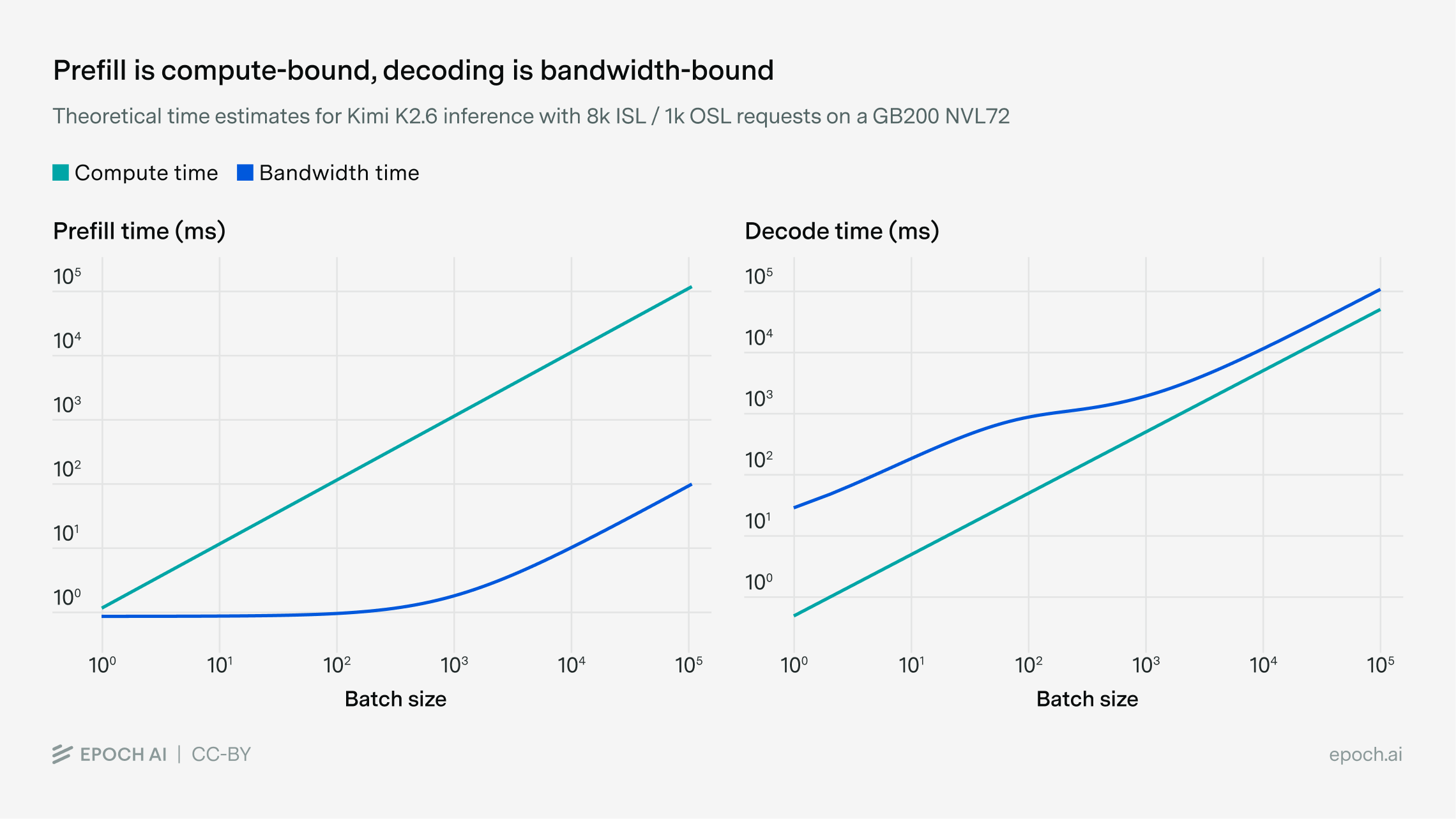
If we plot our expressions for compute and bandwidth time in each of prefill and decode, we can see that prefill is dominated by compute time at all batch sizes, while decoding is dominated by bandwidth time:6
Chunked prefill
So far, we’ve found that for 8,000:1,000 requests, prefill is compute-bound and takes 1B ms per batch, while decoding is bandwidth-bound and takes 868 + 0.5B ms per batch.
As it turns out, we can make use of the fact that compute is sitting idle while we are bandwidth-bound, and bandwidth is idle while we are compute-bound. A common trick to make use of these idle resources is known as chunked prefill. The basic premise is that while you are bandwidth-bound during decoding, you can use your spare compute to start work on the next batch’s prefill computations.
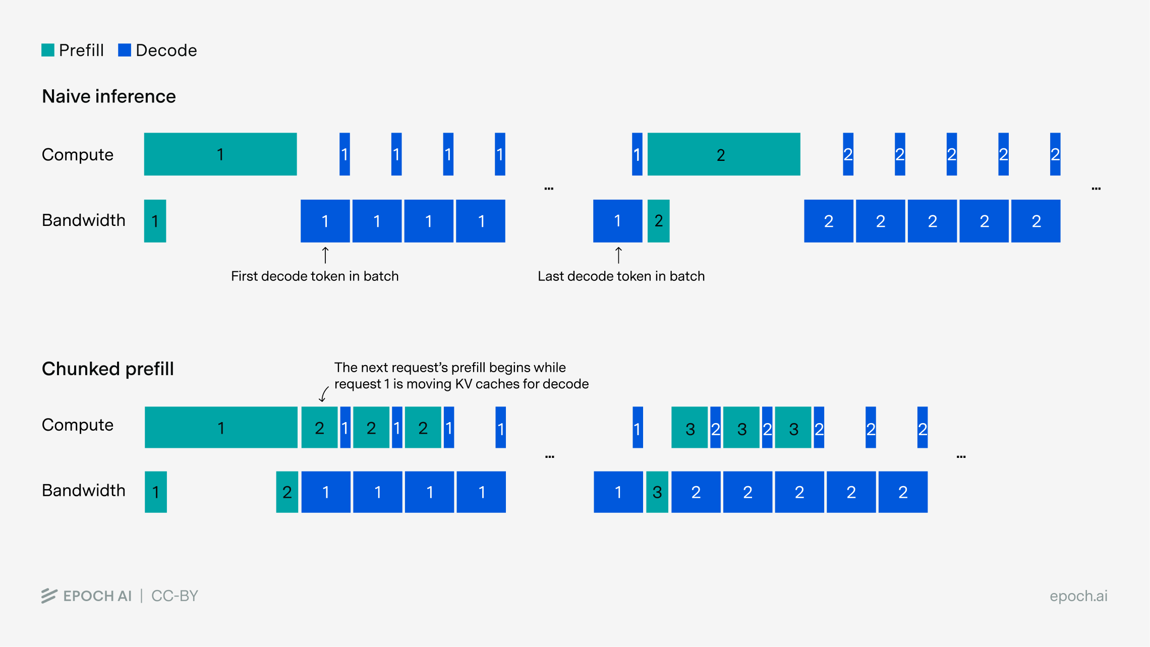
The effect of this overlap is that total time to complete a batch ends up being the larger of total compute time and total bandwidth time, across both prefill and decode.7 The intuition here is that if compute and bandwidth can run concurrently, total time is limited by whichever has more total work to do.
Equivalently,
The final throughput is equal to the batch size times the output length, divided by the time it takes to complete a cycle.
This means the throughput grows monotonically, amortizing the weight loading, until you reach a batch size around ~870 concurrent users per GB200 NVL72. From that point on, inference is compute-bound, and there are no more throughput gains to more batching. In fact, larger batch sizes reduce the speed at which you can serve tokens to each user (the ‘interactivity’). This is because the time to complete a full batch increases in proportion to the number of users, but each user gets only their fixed 1000 tokens of output during that time.
We can also look at the effect of context length. Like many attention mechanisms, MLA’s compute costs grow quadratically with context length, so longer input sequences tend to increase compute costs faster than bandwidth costs. This means that the crossover batch size where throughput becomes compute-bound shrinks as context length increases. For instance, at a context length of 25,000 tokens, the critical B shrinks from 869 to 130.
Speculative decoding
Let’s look at one more trick that gives inference extra juice. Speculative decoding is a technique that uses a small “draft” model to propose candidate tokens several steps ahead,8 which the main model then verifies in a single forward pass. If the main model’s parallel predictions match the draft model’s autoregressive ones, the tokens are accepted.
It’s likely that most major API providers use speculative decoding, since it results in faster inference at minimal cost. This is because the draft model is small enough that its bandwidth and compute overheads are negligible, while each accepted token means one fewer forward pass required by your main model. The one additional cost is that each forward pass on the main model must now predict multiple tokens ahead in parallel, increasing the arithmetic intensity of decoding. For that reason, speculative decoding only helps throughput when decoding is bandwidth-limited. Using state-of-the-art implementations, decoding throughput at a fixed batch size rises by a factor of 3. Since speculative decoding doesn’t help with prefill, the total effect on throughput is closer to 1.6–2×.
Beyond allowing for more throughput at a fixed batch size, speculative decoding can also affect the optimal batch size. By increasing the arithmetic intensity of decoding, speculative decoding reduces the batch size at which decode starts to become compute-bound (after which point there is no reason to further increase batch size, as mentioned in the previous section). For this reason, speculative decoding tends to decrease the optimal batch size.
Putting everything above together, we estimate that the throughput of a B200 NVL72 serving Kimi K2.6 with an 8,000:1,000 profile is around 610,000 tokens per second (tok/s), and aggregate throughput across all chips is 36 billion tokens per second.
Calibrating against inference benchmarks
We’ve built up a fairly rich theoretical model, but we’ve made a few simplifying assumptions, ignoring things like communication latencies, inter-chip bandwidth, and software inefficiencies. To account for these simplifications, we introduce three free parameters:
Compute efficiency: even during large matrix multiplications, it is rare to achieve 100% of a GPU’s stated maximum FLOP/s. This only affects compute-bound stages.
Bandwidth efficiency: similarly, bandwidth rarely operates at peak specifications. Because we don’t explicitly model inter-GPU communication, this parameter will also capture time spent moving activations between GPUs.
Per-step latency: captures a bunch of things like communication latency, kernel scheduling, routing imbalances, and more. This has a larger effect at small throughputs, since we model it as a fixed overhead regardless of batch size.9
SemiAnalysis’s InferenceX dashboard provides data across thousands of inference experiments, which we can use to calibrate these parameters. InferenceX data documents parameters like the total number and type of GPUs used, parallelism strategies, batch size, input and output lengths, model precisions, and more. For any given experiment, we can predict time to first token (TTFT) and time per output token (TPOT) using our theoretical model, and compare to real-world performance. We calibrate our inference model using 111 runs of Kimi K2.5 on Nvidia GPUs across a variety of settings.10
Because the three parameters we’ve introduced have different effects depending on batch size and on what is bottlenecked, we can exploit the variation in experiments to fit these as free parameters, minimizing the discrepancy between our model and the real-world data.11 Doing so, we find estimates of 65% compute efficiency, 30% bandwidth efficiency, and 5ms per-token latency. These are broadly plausible — bandwidth efficiency is lower than expected, but also includes the unmodeled effects of inter-GPU communications.12
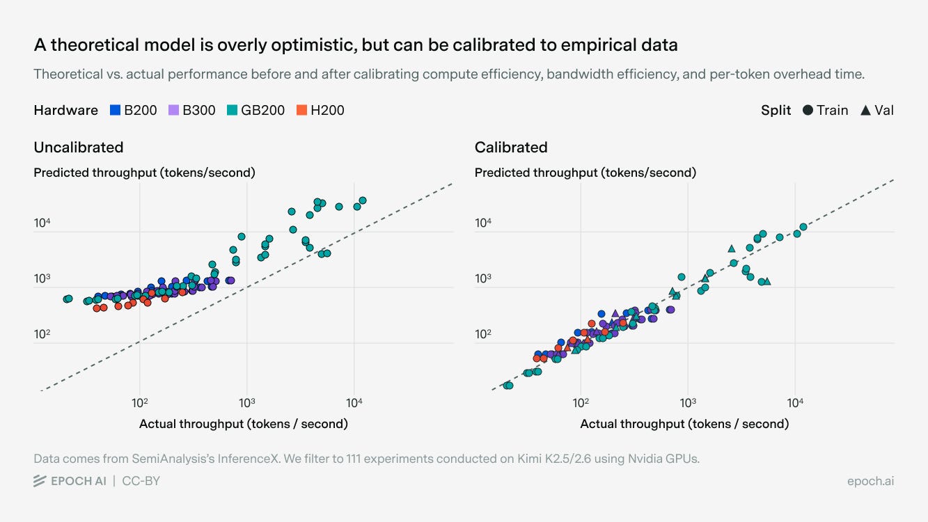
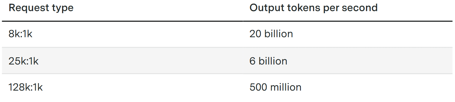
Accounting for these inefficiencies reduces our per-GB200 NVL72 throughput from 640,000 tok/s to 400,000 tok/s.13 Applying the same factors to GB300 systems and then scaling up by the total number of systems produces the following estimates:
The present and future of inference
Our final estimate suggests the world’s Blackwell GPUs could currently deliver a combined 500 million to 20 billion output tokens per second, or between 150,000 and 7 million tokens per month for each person on earth. To put that in perspective, Google, which is likely the most avid token producer today through Google Search summaries, recently claimed that it was serving 1.2 billion tok/s across all its platforms (very likely including both input and output tokens). If we assume a ratio of 8,000:1,000 input to output tokens (many of these requests are presumably short-input search results), they would be serving around 130 million output tokens per second. This suggests that even if we lavishly insist upon serving every Google request with an expensive, trillion-parameter model, there is plenty of inference capacity to serve all the needs of their users.
In fact, it would not only be enough to serve Google, but all tokens worldwide. Exponential View estimates the total tokens processed across all providers at 40 quadrillion tokens per quarter, i.e., around 5 billion tokens per second, four times Google’s traffic. There would still be enough compute capacity to serve all these tokens with a Kimi K2.6-like model, at least in our short- and medium-context settings.
And through a combination of infrastructure deployment and more efficient chips, inference capacity is growing over time. The two relevant trends to track are growth in compute capacity and in memory bandwidth, which are growing exponentially at 3.4×/year and 4.1×/year, respectively. In the long term, the slower-growing factor will determine the overall growth of inference capacity — in this case, compute. In the short term, growth can be closer to 4.1×/year while memory bandwidth remains the primary bottleneck; this will particularly affect long context requests like those in software engineering, since those are more deeply memory-bound. In practice, when we model the growth for short context (8,000:1,000 input-output) and long context (128,000:1,000) inference loads, we find the difference to be minimal; the inference capacity of the world at fixed model size and context length is well modeled as growing at 3.4×/year.
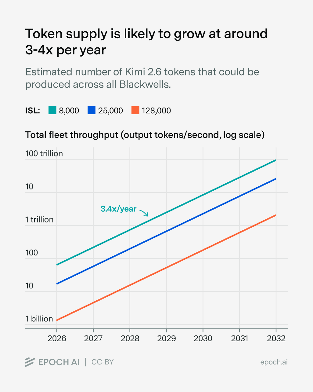
How does this compare to the growth of demand for tokens, at a fixed model size and price? Unfortunately, it’s difficult to make a crisp comparison, but the proxies that we have suggest that demand is growing much faster. For instance, both the quantity of tokens processed by Google in the last year, and by all providers according to Exponential View, have been growing by around 10×/year.
From another angle, we can look at token demand from today’s most intensive AI users: software engineers. Recent reports claim that some of Apple’s software engineers are permitted to use up to $300 in tokens per day, which works out to about 5 million output tokens per day with Claude Opus 4.7 API pricing, or 25 million output tokens per day with Kimi K2.6.14 Another point of comparison comes from Meta, whose 85,000 employees used 60 trillion tokens in one month across the organization. That figure included both input and output tokens; assuming a 25,000:1,000 input-to-output token ratio, that would be around 1 million output tokens per day and employee.
There were about 30 million software engineers worldwide as of 2025 (estimates range from 20 million to 50 million), and Stack Overflow’s 2025 survey on AI usage suggested that only around 47% of developers used AI on a daily basis, as of mid-2025. If all SWEs using AI daily were using it as intensely as Meta or Apple, they would demand somewhere between 10 and 350 trillion tokens per day in aggregate, i.e., between 200 million and 4 billion tokens per second. At the longest context sizes of 128,000:1,000, today’s Blackwell chips would struggle to serve all this potential demand for coding agents using models as large as Kimi K2.6. It also seems likely that both the number of developers using AI, and the intensity of their use will continue to grow rapidly.
All of the proxies above are imperfect. We don’t know the composition of those tokens, whether growth is dominated by small or large models, or the increase in context lengths. The prices of many providers have changed significantly over the period, affecting demand.15 And this analysis entirely ignores the very rapid pace of improvement in inference efficiency, which increases the demand for models of fixed scale by improving capabilities, and decreases it by displacing them with smaller models.
Regardless, these proxies suggest very fast growth in demand at fixed model size and price, likely faster than supply is expanding. And this is compounded by trends towards longer-context usage, especially due to coding and other agentic use cases.
If the demand for AI is outpacing the capacity to serve large models, the predictable consequence is that the price of tokens from large models will rise. This suggests a “compute crunch” is near, if not already here. Indeed, Anthropic has taken measures like reducing quotas during peak hours and incentivizing off-time usage in efforts to manage demand.
In a “crunch”, will everyday users be priced out of AI? Not necessarily. We’ve seen very fast growth in inference efficiency. If that continues, current use cases could be served by smaller, more efficiently served models — arguably, this is what has enabled the fast growth in tokens served we’ve seen so far. The largest models could be reserved for the most productive applications, such as coding, where access to the latest capabilities justifies a high per-token price.
We thank David Schneider-Joseph for in-depth feedback. We also thank Dwarkesh Patel, Jean-Stanislas Denain, Josh You, David Owen, Phil Trammel, Nick Merrill, Vassil Tashev and William Gildea.
How representative is Kimi K2.6 of the frontier? It has an ECI of 152, close to what GPT-5 achieved last year in August, but 8 points behind GPT-5.5 from April this year. It is priced in the Moonshot API as $4.00 per million output tokens, 7.5x times cheaper than GPT-5.5 and similar to GPT-5.4 mini. We guess GPT models are served at a 50% gross margin, while Kimi K2.6 is served close to at cost; this would mean Kimi K2.6 is significantly smaller than GPT-5.5, but likely larger than GPT-5.4 mini.
Why these context lengths in particular? OpenRouter’s State of AI report looks at 100T tokens worth of production data, and finds that the average query has an input length of around 6,000, and an output length of around 800. We bump these up to 8,000:1,000, primarily because this is a common request size for inference performance benchmarks, facilitating comparison. The OpenRouter report as well as Artificial Analysis’s PerfBench each provide empirical evidence that average agentic coding requests have input sequence lengths of around 25,000. Anecdotally, coding sessions can easily reach multiple hundreds of thousands of tokens in context (both Claude Opus 4.7 and Gemini 3.1 Pro support context lengths up to 1M), so we also look at a longer 128,000 token input length.
For simplicity, we model requests as single turns; a more complete accounting would look at the more general setting of multi-turn interactions.
Note that we focus on wall-time throughput per user for simplicity. This differs slightly from “time per output token” (TPOT) which look at time per token once decoding has begun.
Since the model is a mixture of experts, if the batch size is small we can sometimes economize on the number of weights loaded by only loading the experts that will actually be needed for the computation. In practice, the batch sizes we will consider will be large enough that this doesn’t make a practical difference.
The plotted bandwidth lines include an extra factor we glide over in our top-level explanation: at small batch sizes, mixture-of-expert models like Kimi K2.6 do not actually need to load every expert into memory. Between batch sizes under ~100, there is a period of “expert drafting”, where each extra user added to the batch increases the expected number of experts which tokens must be routed to.
This is a bit of a simplification. At the lowest level, the overlap is achieved by appending a chunk of prefill tokens to a decode request. Unfortunately, this only works cleanly for linear MLP layers – attention calculations each have their own KV caches with different dimensions, and you can’t easily append requests. As a result, attention calculations have to be launched as separate kernels after the mixed prefill/decode MLP kernels, so that the total time to process using chunked prefill ends up being the longer of MLP compute or MLP bandwidth (across both prefill and decode), plus the time it takes to do attention operations (the longer of compute or bandwidth for each of prefill and decode). This has a fairly minimal effect at 8,000 token ISL, but becomes more important at longer context lengths. We incorporate the more detailed calculation in all of our numbers.
These days, it may be more common to use integrated Multi-Token Prediction heads (MTP), instead of separate draft models. MTP heads are additional modules built into the model itself, trained for this purpose. The effect is the same either way.
Introducing a per-step latency tends to increase the optimal batch size, since it introduces a fixed cost which can be amortized across users.
At a technical level, we minimize a loss of the form: median_TPOT(|log(pred/actual)|) + median_TTFT(|log(pred/actual)|). We optimize the fit for medians, since outliers may be caused by poorly-configured experiments.
Our simple calibration model ignores several effects that will be absorbed into our parameters, muddying their interpretation. In particular, each parameter is fitted as a single value, regardless of variation in hardware setup or model; some chips may get better or worse utilization due to variation in kernel optimizations, and per-step latencies probably depend on things like model size and chip interface specs.
While our theoretical model overestimates InferenceX experiments by 5× on average, the bias is smaller at higher throughputs, and the largest throughput experiments for Kimi K2.5/2.6 on InferenceX are substantially smaller than the full NVL72 system that we’re basing our headline numbers on.
Assuming a 25,000:1,000 ISL:OSL ratio and that 80% of input tokens are at cache read prices.
Subscriptions by major providers have mostly stayed at the same nominal price, with more expensive tier options introduced, e.g., the $200 ChatGPT Pro subscription complementing the $20 ChatGPT Plus subscription. However, API prices have decreased significantly even for better models. For example, Claude 3.5 Sonnet was half as expensive as Claude 2, and GPT-4o was 4-6x cheaper than GPT-4 on launch.
I always appreciate these analyses!
I think the "forty times Google’s traffic" metric is off. Google recently reported 3.2 quadrillion tokens per month, or 9.6Q per quarter. The Exponential View industry-wide figure for Q1 was 38Q, which is about 4x Google, not 40x. (All things considered, it would be surprising if Google was only 1/40th of worldwide token usage!)
Hello
Thanks for this amazing study. Of course you made a lot of assumptions, but still it gives an idea!
I have a few question from a non specialist :
- Did you take into account CHINA's fast exploding Token consumption ?
https://substack.com/@exponentialview/note/c-265340432?r=18nsoq&utm_source=notes-share-action&utm_medium=web
- I've read that there maths don't add between - token spend as expressed by hypersacaler company Vs. Actual energy expenditure. Is it possible that you minimize by far the compute energy spent elsewhere than in engineering and coding companies (such as AI inside all tools, seach engines, electronic devices, cars.. etc. ?)
Thanks for your time